23 Graphics Environment

The GEOS graphics system provides many powerful tools to enhance your geode’s appearance and graphical capabilities.

The kernel automatically displays much of what appears on the screen. Generic and Visual objects display themselves, so if these objects can display everything your geode needs, you can probably skip this section for now. On the other hand, geodes with any kind of specialized display needs will need imaging code, as will any geodes that print.

This, the first chapter of the Imaging Section, explains the thinking behind the graphics system and the work you’ll have to get done ahead of time to set up the space you’re going to be drawing to. For actual drawing commands, see “Drawing Graphics,” Chapter 24.

Before reading this chapter, you should be familiar with the basics of the generic UI and messaging. You may also want to review high school geometry.

23.1 Graphics Road Map

Graphics is a big topic. It has many applications and thus many ways to apply it. If you will be writing graphics-intensive programs, you’ll probably end up reading everything in these chapters. Chances are, however, that you’ll only need to learn a few things about the graphics system.

This section is for those people who would like to skip around the GEOS imaging system. It contains an outline of the chapter as well as a list of definitions for terms that will be used throughout.

23.1.1 Chapter Structure

This chapter is divided into sections. Which sections you’ll want to read depend on what you’re interested in.

**Road Map
You’re reading the road map now.
Goals
This section goes into the design philosophy behind the GEOS graphics system.
Architecture
The Graphics Architecture section describes the basics behind how the graphics system works.
How to Use Graphics
This section is for programmers new to GEOS who know what sort of graphics they want their geode to have but don’t know how to get it. This section discusses the different contexts in which graphics appear and how you can work within each of those contexts. After going through the section, you may wish to return to this road map to find out where to read more about whatever sort of graphics you’ll be working with.
Coordinate Space
The GEOS graphics system describes locations and distances using a rectangular grid coordinate system. This section explains how to work with and manipulate this space.
Graphics State
This section describes the GState, a data structure used in many contexts and for many purposes throughout the graphics system.
Bitmaps
It is possible to specify an image by using a data structure in which an array of color values is used to represent a rectangular area of the screen. This section describes how such a data structure can be manipulated.
Graphics Strings and Metafiles
This section describes how to create and draw Graphics Strings, also known as GStrings. (See the Vocabulary section, below, for a simple definition of GString.)
Graphics Paths
The graphics system allows you to specify an arbitrary area of the display which can be used in powerful graphics operations. This section explains how to set up a path, a data structure describing the outline of the area you want to specify.
Video Drivers
Most programmers can safely skip this section, but video game writers might want to read it. This section includes some advanced techniques for getting faster drawing rates.
Windowing and Clipping
This section explains some of the work the graphics system does to maintain windows in a Graphical User Interface. Included is an in-depth look at clipping, along with some commands by which you can change the way clipping works.

23.1.2 Vocabulary

Several terms will crop up again and again in your dealings with graphics. Many of these terms will be familiar to programmers experienced with other graphics systems, but those not familiar with any of these terms are encouraged to find out what they mean.

GState, Graphics State
The graphics system maintains data structures called Graphics States, or GStates for short. GStates keep track of how a geode wants to draw things: the colors to use, current text font, scaling information, and so on. Most graphics routines, including all routines that actually draw anything, take a GState as one of their arguments. Thus to draw the outline of a red rectangle, you would first call the GrSetLineColor() routine to change the color used for drawing lines and outlines to red. Only after thus changing the GState would you call the GrDrawRect() command.

Standard Coordinate Space, Document Coordinate Space
Drawing commands in GEOS use the standard coordinate space, also known as the document coordinate space. This is a rectangular grid used for expressing locations and distances. This grid uses units of 1/72nd of an inch. Thus, drawing a point to (72, 72) will draw the point one inch to the right and one inch below the top left corner of an ordinary Content or document.

GString, Graphics String, Metafile
GString is short for Graphics String. A GString is a data structure representing a sequence of graphics commands. Graphics Strings are used many places in the system. GStrings are used to pass graphics through the clipboard. They serve as the descriptors of graphical monikers, which are in turn used as application icons. The printing system uses GStrings to describe images to be printed. A graphics Metafile is just a file containing a GString, taking advantage of this data structure to store a graphics image to disk.

Bitmap
A bitmap is a picture defined as a rectangular array of color values. Note that since display devices normally have their display area defined as a rectangular grid for which each pixel can have a different color value, it is relatively easy to draw a bitmap to the screen, and in fact the graphics system normally works by constructing a bitmap of what is to be displayed and displaying it. Bitmaps are sometimes known as “raster images.”

Path
Paths provide a precise way to specify arbitrary areas of the display area. Like GStrings, they are described by a sequence of drawing commands. Instead of defining a picture, these commands describe a route across the graphics space. The enclosed area can be used in a variety of operations.

Region
Regions provide another approach to describing arbitrary display areas. Regions use a compressed scan-line data structure to represent a pixel-based shape on the display. Though lacking the mathematical precision of paths, region-based operations are very fast and thus ideally suited to certain simple tasks.

Palette, RGB Values
Many display devices can display a wide variety of colors. Of these, most cannot display all their colors at once. Typical configurations can show 16 or 256 colors at a time out of a possible 256K. A palette is one of these subsets of the set of possible colors. When drawing something in color, normally the color to draw with is specified by the palette index, that color’s place in the table. The value stored in each entry is an RGB value, a color described in terms of its red, green, and blue components. Each of these three values ranges between 0 and 255. Geodes can change the RGB values associated with palette entries and thus change the available colors.

Video Driver
These geodes stand between the graphics system and the actual display device. They maintain device independence and do a lot of the “behind the scenes” work of the graphics system.

Windowing, clipping, “marked invalid”
The windowing and graphics systems are heavily intertwined. The graphics system controls how windows should be drawn, while the windows system keeps track of which parts of various displays are visible. For the most part graphics programmers don’t have to worry too much about the windowing system, but there are some terms worth knowing. Clipping is the process of keeping track of what things drawn to a window are actually visible. If a geode draws something beyond the edge of a window, the system can’t just ignore the drawing, as the user might later reveal the drawing by scrolling onto that area. The graphics system “clips” the graphic, being sure to show only those parts that are in the visible part of a window. Further clipping takes place when a window is obscured behind another window. Any drawing on the lower window must not show up until the upper window is moved. The “clipping region” is that area of a window which is visible-anything drawn to the window outside the region will be clipped (see Figure 23-1). Programs can reduce the clipping areas of any of their associated windows.

Figure 23-1 Clipping
Clipping is the process of determining what needs to be drawn. If something appears outside the bounds of its window or is hidden under another window, the system should not draw it. The clipping region is the area of the display where things will be drawn: in the window, but not obscured. In the figure, the shaded area shows the clipping region.

The windowing system is able to work much more quickly by assuming that not too many things are going to be changing at once. Normally it can assume that a given area of the screen will look like it did a short while ago. When it’s time to change an area of the screen, that area is said to be “marked invalid,” since whatever is presently being shown there is no longer valid. The normal example is that if a pull-down menu has been obscuring part of a document, when the menu goes away, the part of the document that becomes visible must be redrawn.

MSG_VIS_DRAW, MSG_META_EXPOSED
These messages are sent to visible objects to instruct them to redraw themselves; if you are using graphics to display a visible object then you are probably intercepting MSG_VIS_DRAW. MSG_META_EXPOSED lets an object know that it has been marked invalid; either it has to be drawn for the first time, or part or all of it has been exposed (hence the name). The UI controller sends this message to the top object in the Vis hierarchy. MSG_VIS_DRAW, on the other hand, specifically instructs an object to redraw itself. Generally, a Vis object will respond to MSG_META_EXPOSED by sending MSG_VIS_DRAW to itself; it responds to MSG_VIS_DRAW by issuing the appropriate drawing commands, then sending MSG_VIS_DRAW to each of its children.

Graphic Objects
Graphic Objects provide the user with an interface for working with graphics in a manner similar to GeoDraw’s. They are useful for programs which allow the users to construct some sort of graphical document or provide a sort of graphical overlay for a spreadsheet.

23.2 Graphics Goals

The graphics system is in charge of displaying everything in GEOS. Thus, it is vital that the GEOS graphics system be both powerful and easy to use. Features such as outline font support and WYSIWYG printing, usually afterthoughts on other operating systems, have been incorporated into the GEOS kernel. The graphics system was designed to be state of the art and thus had to achieve several goals:

Fast Operation The GEOS graphics system is heavily optimized for common operations on low-end PCs. To allow a windowing system to run on an 8088 machine, it is vital that line drawing, clipping, and other common graphical operations run very quickly. They do.
Device Independence Applications are sheltered from the hardware. Coordinate system units are device independent so that all of your drawing commands use real-world measurements. These units are then translated into device coordinates by the kernel.
Complete Set of Drawing Primitives The graphics system must be able to draw a wide variety of shapes and objects to meet the needs of the UI and applications. It does.
Built In Support for Outline Fonts GEOS includes outline font technology supporting a variety of font formats. Outline fonts are text typefaces which are defined by their outline shape rather than by a bitmap representation. Outline fonts can be scaled with no apparent loss of smoothness. GEOS also supports bitmap-based fonts; however the very nature of these fonts makes them non-WYSIWYG.
Single Imaging Model for Screen and Hardcopy The graphics system uses the same high level graphics language for screen imaging as for printing. Because the GEOS system creates both screen and printed images through the same language, the screen can display a document just as it will be printed. Except for differences in resolution, what you see is what you get.

23.3 Graphics Architecture

The graphics system involves many pieces of GEOS working together to turn an application’s UI and graphics commands into drawings on a display.

The graphics portion of the kernel automatically makes any requested transformations to the coordinate space dealing with scaling, rotation, etc. It transforms complicated drawing commands into simpler ones supported by the video drivers. (See Figure 23-2.)

Figure 23-2 Graphics System Architecture

The video driver can render these simplified commands directly on the device. The video driver checks for collisions, making sure that if whatever is being drawn coincides with the mouse pointer, the mouse pointer will be drawn on top. The video driver does clipping so a geode doesn’t draw outside its window.

Commands and information flow in this manner from application to the Video Device, though information also flows in the opposite direction, so that the kernel can get information about the display device’s resolution, size, and capabilities.

If the geode is going to draw text, the graphics system makes calls to the font manager. If the requested font isn’t already in memory, the font manager loads it. The font manager then makes calls to the individual font driver for information about specific characters.

23.4 How To Use Graphics

When looking at the source code of sample applications, it’s usually not too hard to pick out the commands that do the actual drawing. Commands with names like GrDraw…() generally are self-explanatory. It’s not so easy to pick out the commands that set up an area in which the drawing will take place. Part of the problem is that there are many ways to display graphics; each is well suited for different tasks. This section of the chapter provides some practical knowledge about the various ways to display graphics and which situations are appropriate for each.

When possible, the best way to learn how to perform a graphics action is to look at code which performs a similar action. The sample program presented in “First Steps: Hello World,” Chapter 4 shows a simple graphics environment sufficient for many geodes. If you only need to change what is being displayed (as opposed to how it is displayed), you can work straight from the example, drawing different shapes using commands found in “Drawing Graphics,” Chapter 24. Most basic graphics techniques are used in one sample program or another. By combining and adapting code from the sample programs, you can take care of most simple graphics needs.

If you can’t find a sample geode to work from, there are several points to consider when deciding what sort of graphics environment to set up.

Sometimes the only graphics commands in a geode will be those used to define that geode’s program icon. This is a common enough case that instructions for setting up your geode’s icon are in the program topics section, section 6.2 of chapter 6.
Will existing generic UI gadgetry be sufficient for everything you want to display? If you’re writing a utility, it might be. If you’re writing an arcade game, it probably won’t be.
If your geode will be displaying graphics, will the user ever interact directly with the graphics? A graphing program might draw a graph based on data the user types in. Such a program could draw the graph but might not actually allow the user to interact with the graph. On the other hand, an art program will probably expect the user to interact with the graphics directly.

Once you’ve figured out just what your geode’s graphical needs are, you’re ready to find out which pieces of graphics machinery are right for you.

For custom graphics that will appear in a view, the content object of the GenView must be prepared to issue graphics commands. A common tactic is to create a subclass of VisContentClass and let an object of this subclass act as the content for a view. The subclass would very likely have a specialized MSG_VIS_DRAW. The Process object is another popular choice for the view’s output descriptor. In this case, the process must be prepared to intercept any messages the view is likely to send, with MSG_META_EXPOSED and MSG_VIS_DRAW of the most interest. Whichever object, process or content, is the content of a view can respond to MSG_META_EXPOSED or MSG_VIS_DRAW by calling kernel graphics routines. For more information on how to use these objects, see “GenView,” Chapter 9 of the Object Reference Book.

Geodes that wish to allow the user to edit graphical elements would do well to incorporate a Graphic Object into their hierarchies. These objects have considerable power and include UI to allow the user to work graphics within them. See “Graphic Object Library,” Chapter 18 of the Object Reference Book for more information about these object classes.

As you learn more advanced graphics concepts you may discover shortcuts. As you get deeper into graphics, you should keep a cardinal rule in mind. Any time the graphics space is obscured and then exposed, the geode must be able to draw correctly, no matter what changes have been made. If your geode only draws on a MSG_VIS_DRAW, it will automatically follow this rule. However, applications using shortcuts must take MSG_VIS_DRAW into account; it may be sent at any time, and what it draws may wipe out what was there before. An arcade game that moves a spaceship by blitting a bitmap may be fast; however, be sure that the spaceship will be drawn to the right place if the game’s window is obscured and then exposed. Don’t worry if this sounds confusing now, but keep these words in mind as you read on.

23.5 Coordinate Space

The graphics system uses a rectangular coordinate grid to specify the size and position at which drawing commands will be carried out. This is a logical choice as most display devices use a rectangular grid of pixels. “Smart” devices with built in graphics routines tend to use coordinate grids to set place, size, and sometimes movement. “Dumb” devices, capable only of displaying bitmaps, always have these bitmaps described in terms of pixels on a square grid. The GEOS graphics system expects the geode to use the provided device-independent grid to describe graphics commands (see Figure 23-3). The graphics system will then convert this information to device coordinates: coordinates set up for the specific display device, using a grid of pixels.

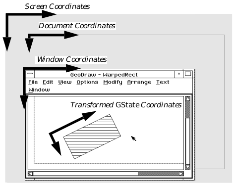
Figure 23-3 Coordinate Spaces
At any one time, the graphics system keeps track of several coordinate spaces. You only have to worry about the coordinate spaces for the GState you are working with; GEOS takes care of the rest.

23.5.1 Standard Coordinate Space

The standard coordinate space is what the application uses to describe where things are to be drawn. It is device independent, based on real world units: typographer’s points, about 1/72nd of an inch. The origin of the coordinate system is normally the upper left corner of the document, but this can change with context and with changes made by the kernel or even your geode. The coordinate space normally extends from -16384 to 16383 horizontally and vertically. These constants may be referenced as MIN_COORD and MAX_COORD. Note that if you’re going to be printing your document, you should restrict yourself to coordinates between -4096 to +4096 to account for scaling to draw on high resolution printers. It is possible to define a 32-bit coordinate space, which gives more room but costs speed and memory. For details about 32-bit spaces, see section 23.5.5.

Whenever you draw something, you must specify the coordinates where that thing will be drawn. The coordinates you pass specify where in the coordinate plane that thing will be drawn; the plane, in turn, may be translated, scaled, and/or rotated from the standard window coordinate system (see section 23.5.2).

The system also maintains a device coordinate system, with a device pixel defined as the unit of the grid. This is the type of coordinate system most programmers are used to, but it is certainly not device independent. The graphics system will do all the worrying about device coordinates so your program doesn’t have to. (Note, however, that GrDrawImage(), GrDrawHugeImage(), and GrBrushPolyline() are more device-dependant than most routines; see section 24.2.10 of chapter 24 and section 24.2.8 of chapter 24 for information on these routines).

Standard GEOS coordinates depart from the device model, taking an approach closer to a pure mathematical Cartesian plane. Programmers used to working with device-based coordinates are especially encouraged to read section 23.5.4 to learn about some of the differences.

23.5.2 Coordinate Transformations

GEOS provides routines which “transform” the coordinate space. These commands can shift, magnify, or rotate the coordinate grid, or perform several of these changes at once (see Figure 23-4). These transformations affect structures in the GState, and new transformations can be combined with or replace a GState’s current transformation.

Figure 23-4 Effects of Simple Transformations

These transformations apply to the coordinate space, not to individual objects. As a result, if you apply a 200% scaling factor to a drawing not centered on the origin, not only will its size change, but its position will change as well. If you want these operations to affect an object but not its position, you should translate the coordinates so that the origin is at the desired center of scaling or rotation, apply the scaling or rotation, draw the object at the translated origin, then change the coordinates back. For an example of this sort of operation, see Figure 23-5.

Figure 23-5 Rotating an Object About Its Center
Remember that transformations apply to the whole coordinate space, their effects based around the origin. Thus, to draw a rotated shape at certain coordinates, if the space is rotated before drawing, the coordinates at which the shape will be drawn will be rotated about the origin as well. There is a simple way to draw a shape rotated about an arbitrary axis. First, apply a transformation so that the origin is at the planned center of rotation. Next, apply the rotation. Finally, draw the figure at the new origin.

Since they are stored in the GState, these transformations endure-they do not go away after you’ve drawn your next object. If you apply a 90 degree rotation, you will continue drawing rotated to 90 degrees until you either rotate to some other angle or use another Graphics State. Transformations are also cumulative. If you rotate your space 30°, then translate it up an inch, the result will be a rotated, translated coordinate space. If you want to nullify your last transformation, apply the opposite transformation.

When applying a new transformation to a space which has already been transformed, the old transformations will affect the new one. Be careful, therefore, of the order of your transformations when combining a translation with any other kind of transformation. If you make your transformations in the wrong order, you may not get what you expected (for an example, see Figure 23-6).

Figure 23-6 Ordering Transformation Combinations
When combining translations with other transformations, remember that the order of the transformations becomes important. The drawing on the left was rotated and then translated. The drawing on the right received the same transformations but in reverse order. Note that the drawings ended up being drawn to different positions.

23.5.2.1 Simple Transformations

GrApplyRotation(), GrApplyScale(), GrApplyTranslation(), GrSetDefaultTransform(), GrSetNullTransform(), GrInitDefaultTransform(), GrSaveTransform(), GrRestoreTransform()

If you find yourself using transformations at all, they will probably all be rotations, scalings, and translations. The GEOS graphics system includes commands to apply these kinds of transformations to your coordinate system, taking the form GrApplyTransformation(). These commands work with a transformation data structure associated with the Graphics State, so everything drawn in that Graphics State will be suitably transformed. Figure 23-4 illustrates the effects of these transformations.

GrApplyRotation() rotates the coordinate space, turning it counterclockwise around the origin. All objects drawn after the rotation will appear as if someone had turned their drawing surface to a new angle. With a 90° rotation, a shape centered at would draw as if centered at. Anything drawn centered at the origin would not change position but would be drawn with the new orientation.

GrApplyScale() resizes the coordinate space; this is useful for zooming in and out. After applying a scale to double the size of everything in the x and y directions, everything will be drawn twice as big, centered twice as far away from the origin. Applying a negative scale causes objects to be drawn with the scale suggested by the magnitude of the scaling factor but “flipped over” to the other side of the coordinate axes.

GrApplyTranslation() causes the coordinate system to be shifted over. After a translation, everything will be drawn at a new position, with no change in orientation or size.

To undo the effects of a transformation, you can apply the opposite transformation: rotate the other way, translate in the opposite direction, or scale with the inverse factor.

To undo the effects of all prior transformations, return to the default transformation matrix using the GrSetDefaultTransform() command. The routine GrSetNullTransform() sets the Graphics State transformation to the null transform-nullifying not only your transformations, but any the system may have imposed as well. For the most part, you should avoid using the GrSetNullTransform() command and use the GrSetDefaultTransform() instead. You can change the default transformation matrix using GrInitDefaultTransform(), but this is generally a bad idea since the windowing system works with the default transformation, and if a geode begins making capricious changes, this can produce strange images.

There are “push” and “pop” operations for transformations. To keep a record of the GState’s current transformation, call GrSaveTransform(). To restore the saved transformation, call GrRestoreTransform().

23.5.2.2 Complicated Transformations

GrApplyTransform(), GrSetTransform(), GrGetTransform(), GrTransformByMatrix(), GrUntransformByMatrix()

You may want to make some change to the coordinate system that has no simple correspondence to scaling, rotation, or translation. Perhaps you know some linear algebra and want to use your knowledge to combine several transformation functions into a single transformation (thus improving execution speed). All transformations on the coordinate system are expressed in the form of transformation matrices. A GEOS graphics system transformation consists of a matrix containing 6 variables and 3 constants (see Equation 23-1). The six variables allow for standard coordinate transformations. The constants (0, 0, and 1 respectively) allow these transformation matrices to be composed. For example, multiplying a scaling matrix with a rotation matrix creates a matrix which represents a combined scaling and rotation. The six variable matrix elements are stored in a TransMatrix structure.

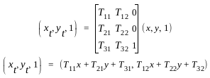
Equation 23-1 Transformation Matrices
The left hand side shows the new coordinate pair resulting from applying the transformation to the old coordinates. The right hand side of the equation shows the formula used to compute these new coordinates. The “1” following each coordinate pair is a constant to allow matrix multiplications.

The GEOS system uses one matrix to store the Graphics State transformation and one to store the Window transformation. When told to apply a new transformation, the graphics system constructs a matrix to represent the requested transformation change and multiplies this matrix by the old transformation matrix. To combine these matrices, GEOS multiplies them together to get the cross-product (See Equation 23-2).

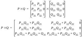
Equation 23-2 Combining Transformations
Transformations are combined by taking the cross product of their matrices. In cases where order is important, the leftmost factor represents the more recent transformation.

If you know that there’s a particular combination of transformations you’re going to be using a lot, you can do some math in advance to compute your own transformation matrix, then apply the raw matrix as a transformation using GrApplyTransform(). Equation 23-3 shows the matrices corresponding to the simple transformations. To replace the GState’s current transformation matrix with the matrix of your choice, use GrSetTransform(). To find out the current transformation, call GrGetTransform().

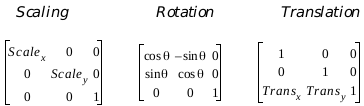
Equation 23-3 Matrices for Standard Transformations

GrTransformByMatrix() returns the results of transforming a passed coordinate pair using an arbitrary transformation matrix. GrUntransformByMatrix() performs the reverse operation, returning the coordinates which would have transformed to the passed coordinates.

Sometimes you have to be careful about the order in which these transformations are supposed to occur. When multiplying transformation matrices together, the transformation that is applied later is the first in the multiplication pair. You can combine any number of rotations and scalings together without having to worry about order: the resulting matrices will be the same. When combining a translation with any other kind of operation, it makes a difference what order you make the transformations and thus makes a difference based on what order you multiply the matrices (See Figure 23-6 and Equation 23-2).

23.5.3 Precise Coordinates

As has been previously stated, coordinates are normally given in typographer’s points. Most graphics commands accept coordinates accurate to the nearest point. This should be more than sufficient for most geodes, but for those specialized programs, more precise drawing is possible.

For simple cases, it is possible to create precise drawings by scaling the drawings. To make drawings accurate to one fourth of a point, for example, scale by 25% and multiply all coordinates accordingly. However, this approach is limited and may result in confusing code.

Another way to make precise drawings is to use the graphics commands which have been specially set up to take more precise coordinates. These commands will not be described in detail here, but keep them in mind when planning ultra-high resolution applications. GrRelMoveTo(), GrDrawRelLineTo(), GrDrawRelCurveTo(), and GrDrawRelArc3PointTo() take WWFixed coordinates, and are thus accurate to a fraction of a point. To draw a precise outline, use these commands to draw the components of the outline. To fill an area, use the precise drawing commands to describe the path forming the outline of the area, then fill the path.

23.5.4 Device Coordinates

Most programmers can work quite well within the document space regardless of how coordinates will correspond to device coordinates. However, some programmers might need to know about the device coordinates as well. The system provides clever algorithms for going from document to device space for all programmers, as well as routines to get device coordinate information from the device driver.

23.5.4.1 What the System Draws on the Device

Consider a device whose pixels are exactly 1/72nd of an inch, such that no scaling is required to map document units to device units. The relationship of the coordinate systems is illustrated below. Note that a pixel falls between each pair of document units. This is a further demonstration of the concept that document coordinates specify a location in the document coordinate space, not a pixel.

Figure 23-7 Document and Device Coordinates
When using a device with 72dpi resolution, it’s pretty simple to figure out what will be drawn to the device.

Next consider a device that has a resolution of 108 dpi, which is 1.5 times greater than our default 72 dpi. That is, there are 1.5x1.5 pixels on the device for each square document unit. The basic problem here is that the coordinates that are specified in document space map to non-integer pixels in device space. The graphics system would like the pixels to be half-filled along two edges of the rectangle (see Figure 23-8). Unfortunately, a pixel must be either filled or empty, so the system needs a set of rules to follow in this situation. These rules are

If the midpoint of a pixel (i.e., the device coordinate of that pixel) falls inside the area’s boundary, that pixel is filled.
Conversely, if the midpoint of a pixel falls outside the area’s border, the pixel is not filled.
If the midpoint of the pixel falls exactly on the border of the area to be filled, the following rule is used: Pixels on the left or the top are not filled; Pixels on the right or the bottom are filled; Pixels in the left-bottom and top-right corners are not filled.

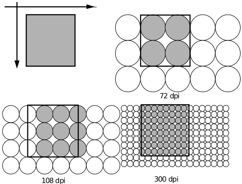
Figure 23-8 Different Device Coordinates
When using a device with a resolution that is not a multiple of 72dpi, GEOS has to decide which borderline pixels have to be filled.

These rules might seem a little odd: Why not just fill all the pixels that would be touched by the area? One of the problems with this approach is that areas that did not overlap in the document space would overlap on the device. Or more specifically, they would overlap only on some devices (depending on the resolution), which is even worse. The rules have the property that adjoining areas in document space will not overlap in any device space.

Our next set of potential problems comes with lines. Lines can be very thin and thus might be invisible on some low-resolution devices. If the graphics system used the rules for filled objects then some thin lines would be only partially drawn on low resolution devices. GEOS uses Bresenham’s algorithm for drawing straight thin lines, ensuring that a continuous group of pixels will be turned on for a line (see Figure 23-9). This continuity is insured due to the behavior of the algorithm:

If the line is more horizontal then vertical, exactly one pixel will be turned on in each column between the two endpoints.
If the line is more vertical than horizontal, exactly one pixel will be turned on in each row.
If the line is exactly 45 degrees, exactly one pixel will be turned on in each column and row.

Figure 23-9 Drawing Thin Lines
If the thin line were drawn as if it were a skinny filled polygon, there would be gaps as shown to the left. Using Bresenham’s line algorithm, GEOS eliminates the gaps, resulting in a continuous line drawn as on the right.

Since ellipses and Bèzier curves are drawn as polylines, Bresenham’s algorithm will work with them.

23.5.4.2 Converting Between Doc and Device Coordinates

GrTransform(), GrUntransform(), GrTransformWWFixed(), GrUntransformWWFixed()

Given a coordinate pair, at times it’s convenient to know the corresponding device coordinates. Sometimes the reverse is true. Use these functions to convert a coordinate pair to device coordinates or vice versa. GrTransform() takes a coordinate pair and returns device coordinates. GrUntransform() does the reverse. If you want to be able to get a more exact value for these coordinates you can use GrTransformWWFixed() and GrUntransformWWFixed(). These return fixed point values so you can do other math on them before rounding off to get a whole number that the graphics system can use.

To transform points through an arbitrary transformation instead of to device coordinates, use the GrTransformByMatrix() or GrUntransformByMatrix() routines, described previously.

23.5.5 Larger Document Spaces

GrApplyDWordTranslation(), GrTransformDWord(), GrUntransformDWord(), GrTransformDWFixed(), GrUntransformDWFixed()

Some applications may need a graphics space larger than the 19 foot square of the standard coordinate space (10 foot square for printed documents). Some spreadsheets can take up a lot of room, as can wide banners. Geodes that will need a large drawing space can request a 32-bit graphics space, i.e. a coordinate space in which each axis is points long (more than 4 billion points, or 900 miles). Most applications will be able to get by with standard 16-bit coordinate spaces, and their authors may safely skip this section. Note, however, that the Graphic and Spreadsheet objects use 32-bit graphics spaces for display.

If a geode will use a 32-bit space in a view, it will need a VisContent object with the VCNA_LARGE_DOCUMENT_MODEL attribute.

For the most part, 32-bit documents use the same graphics commands as regular 16-bit documents. No single drawing command can cover more than a standard document area; each has been optimized to draw quickly in 16 bits. To draw to the outlying reaches of your document space, apply a special translation that takes 32-bit coordinates, then use normal drawing routines in your new location.

A model for working with 32-bit graphics spaces commonly used with spreadsheets is to break the graphics space into sections. To draw anything, the geode first uses a translation to get to the proper section, then makes the appropriate graphics calls to draw within that section. Similarly a GeoDraw-style application might translate to the appropriate page, then make normal graphics commands to draw to that page (see Figure 23-10).

If you wish to display this 32-bit coordinate graphics space to the screen, you’ll probably want to do so in a 32-bit content.

The standard graphics commands can only draw to one 16 bit space at a time. You will need to translate the coordinate space to choose which 16-bit portion of the 32-bit space you want to draw to. To do so you need to use some special translation functions. GrApplyDWordTranslation() corresponds to the GrApplyTranslation() function normally used.You can use this routine to make the jumps necessary to access far away portions of the graphics space. Since a coordinate can now be in a much larger area than before, all routines that deal with a point’s position have 32-bit equivalents.

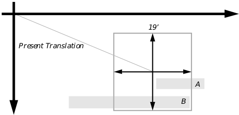
Figure 23-10 Thirty-two Bit Graphics Spaces
When drawing in a 32-bit space, remember that the drawing commands are only prepared to draw in a sixteen-bit subspace. In the figure, rectangle A isn’t entirely within reach of the origin, so it will be necessary to translate the origin again before drawing this rectangle. Rectangle B is not only partially out of reach of the origin, it’s too big to fit inside of a 16-bit space. In order to draw this rectangle, you would have to divide it into two pieces.

GrTransformDWord() and GrUntransformDWord() take the place of GrTransform() and GrUntransform(). GrTransformDWFixed() and GrUntransformDWFixed() take the place of GrTransformWWFixed() and GrUntransformWWFixed(), with two words in the integer part of the number instead of one.

23.5.6 Current Position

GrMoveTo(), GrRelMoveTo(), GrGetCurPos(), GrGetCurPosWWFixed()

The graphics system supports the notion of a current position, sometimes called a pen position. Note that the pen position metaphor predates “pen computing”; please don’t confuse these concepts. The concept behind the pen position is that all graphics commands are executed by a pen that ends up at the last place drawn. So if the last command was to draw a curve ending at (20, 20), the pen will still be there. There are special drawing commands that work with the pen position, so you could then draw a line from the current position to (30, 30). The line would extend from (20, 20) to (30, 30), and the pen would then be at (30, 30).

Calling GrMoveTo() moves the pen position to coordinates of your choice. GrRelMoveTo() moves the pen to a location relative to its present position. GrRelMoveTo() takes coordinates accurate to a fraction of a point, allowing for very precise placement. Call GrGetCurPos() to get the current position, GrGetCurPosWWFixed() to do so with greater accuracy.

There are some guidelines to follow when figuring out where your pen position is going to end up after a draw operation. If you call the GrDrawLineTo() procedure, the pen will end up at the point drawn to. If you call any draw/fill procedure that takes two points as arguments, the pen position usually ends up at the second point passed; if it does not, the reference entry will note where the pen position ends. When text draws at the current position, the current position is used to place the left side of the text. When done drawing the text, the current position has moved to the right side of the text.

23.6 Graphics State

The data structure known as the Graphics State, or GState, keeps track of changes your code makes about how it wants to draw things. If your geode changes its transformation, everything you draw from that point will be drawn transformed until you change the transformation again. If your geode sets the line width to two points, all lines to come will be drawn two points wide until the width is set to something else. Many graphics routines ask that you pass a GState along as one of the parameters so they know where and how to draw what you’ve requested.

23.6.1 GState Contents

Sometimes it’s convenient to think of the GState as being analogous to the Properties boxes in GeoDraw. The GState keeps track of how the program wants to draw lines, text, and filled areas, just as the Line Properties, Text Properties, and Area Properties boxes keep track of how the GeoDraw user wants to draw these objects.

While handy, this analogy doesn’t do the GState justice. The GState keeps track of many things:

Mix Mode The graphics system allows for different mix modes (sometimes known as copy modes). These drawing modes permit the geode to draw in such ways that it erases instead of drawing, draws using the inverse of whatever it’s drawing on, or uses various other modes.
Current Position (also known as Pen Position) The graphics system keeps track of the position of the last thing drawn. If your geode wants to draw something else at this location, there are drawing commands that will draw at the current position.
Area Attributes The GState contains information that the graphics system will use when filling areas. This information includes the color and fill pattern to use.
Line attributes The graphics system uses information stored in the Graphics State to keep track of what color and pattern to use when drawing lines. The GState also keeps track of whether lines should be drawn as dotted, and if so what sort of dot-dash pattern to use. The GState contains the line width. It also contains line join information, which controls how lines will be drawn when they meet at an angle, as at the vertices of a polygon.
Text Attributes The Graphics State contains the ID of the current font, the font size, and the text style. It also contains a color and pattern to use, information about the font, and some esoteric text-drawing options.
Coordinate Space Transformations The GState keeps track of the current coordinate space transformation. If there is an associated window, the window’s transformation matrix is maintained separately with the window’s information.
Associated Window The GState knows the handle of the window associated with the GState. This is the window that will determine where drawings appear and how they are clipped.
Associated GString If the application is building a GString, the GState is aware of it. The GState contains a reference to the GString. When the graphics system turns graphics commands into GString elements, these elements will be appended to the referenced GString.
Associated Path If the application is building a path, the GState contains a pointer to the path along which new path elements are passed, similar to the way GString elements are passed. The GState also keeps track of whether the current path is to be combined with another path or should be used “as is.”
Clipping Information The GState keeps track of clipping information in addition to that maintained by the window.

The function of many of these parts may be fairly intuitive to someone used to working with graphics programs. Some of the others may require additional explanation, especially when it comes to how to work with them.

23.6.2 Working with GStates

GrCreateState(), GrDestroyState(), GrSaveState(), GrRestoreState()

As has been mentioned, most graphics routines require that a GState handle be provided as an argument. Beginning programmers are often unclear on just where to get the GState to use.

Many drawing routines are called by MSG_VIS_DRAW. This message provides a GState, and all routines in the handlers for this message should use the provided GState. Creating a new GState under these circumstances is unnecessary and wasteful. However, sometimes you will need to create a GState. GrCreateState() creates a GState with the default characteristics. You must specify the window with which the GState will be associated.

Commands which change drawing attributes or the current position change the GState.

GrDestroyState() is used to get rid of a GState, freeing the memory to be used by other things. If GStates are created but not destroyed, eventually they will take too much memory. Normally, for each call to GrCreateState() there is a corresponding GrDestroyState(). MSG_VIS_DRAW handlers don’t need to destroy the passed GState. Graphics states are cached so that GrCreateState() and GrDestroyState() don’t normally need to call MemAlloc() or MemFree(). When GStates are freed, their space is added to the cache. When the memory manager needs to find space on the heap, it flushes the cache.

A geode is most likely to call GrCreateState() when about to draw a piece of geode-defined UI. Other than that, you’ll probably be using GStates provided to you by the system. You might want to create a GState if you wanted to calculate something (perhaps the length, in inches, of a text string) when you had no appropriate GState.

GrSaveState() provides a sort of “push” operation that works with GStates. When you call certain functions, like GrSetAreaColor(), new values will wipe out the values of the old GState. But if you’ve previously called GrSaveState(), then any time you call GrRestoreState() on your saved state, it will come back and displace the current state. Your application can save a GState to save a commonly used clipping region, which could then be restored by restoring the state instead of repeating all the operations needed to duplicate the region. GrSaveTransform() and GrRestoreTransform() are optimizations of GrSaveState() and GrRestoreState(), but they only preserve the GState’s transformation.

23.7 Working With Bitmaps

GrCreateBitmap(), GrDestroyBitmap(), GrEditBitmap() GrGetPoint(), GrSetBitmapMode(), GrGetBitmapMode(), GrSetBitmapRes(), GrGetBitmapRes(), GrClearBitmap(), GrGetBitmapSize(), GrCompactBitmap(), GrUncompactBitmap()

Bitmaps are useful for describing complicated pictures that don’t have to be smooth at all resolutions. For example, coming up with all the lines and shapes necessary to describe a complicated photograph would be time-consuming and a waste of memory. It’s much easier to set up a rectangular array of cells and to set a color value for each cell. Bitmaps are often used for defining program icons. GEOS includes a great deal of bitmap support. It has kernel routines to create, modify, and draw bitmaps.

There are three main ways to create a bitmap for an application to use. One often used is to embed the data of a desired bitmap directly into a graphics string. This is the way normally used for defining system icons. The other common way is to call the kernel graphics routine GrCreateBitmap(). Another way to create a bitmap, not used so often, is to manipulate memory directly: The formats used for describing bitmaps are public, and though it would be easier in most cases to work through GrCreateBitmap(), those with specialized needs might want to create their bitmap data structures from scratch.

The GrCreateBitmap() routine creates an offscreen bitmap and returns a Graphics State which can be drawn to; changes to this Graphics State become changes to the offscreen bitmap. For example, calling GrDrawLine() and passing the Graphics State provided with such a bitmap would result in a bitmap depicting a line. To display this bitmap, call the GrFillBitmap(), GrDrawHugeBitmap(), GrDrawImage(), or GrDrawHugeImage() commands in another graphics space (see section 24.2.10 of chapter 24).

When creating a bitmap, you must make choices about what sort of bitmap you want. Depending on your choices, GEOS will be able to use a variety of optimizations. For instance, it takes much less room to store a monochrome bitmap than a color bitmap the same size.

Whenever creating a bitmap, you must specify its dimensions and what sort of coloring it will use (monochrome, four bit, eight bit, or 24 bit).

You may store a mask with your bitmap. This mask works something like the mask used when drawing a view’s mouse pointer. When the bitmap is drawn, blank areas of the bitmap will be drawn as black for those pixels where the mask is turned on. For pixels where the mask is turned off, whatever was underneath the bitmap will be allowed to show through.

By asking for a Complex bitmap, you can specify even more information. Complex bitmaps may include their own palette and may specify their own horizontal and vertical resolution. They are very useful for working with bitmaps that may have been captured on other systems or for working with display devices.

The GrDestroyBitmap() routine destroys some or all of the information associated with a bitmap. You may use this function to free all memory taken up by the bitmap. You may also use this function to free only the GState associated with a bitmap by GrCreateBitmap(), but leave the bitmap’s data alone; the BMDestroy argument will determine exactly what is destroyed. This usage comes in handy for those times when a bitmap will not be changing, but will be drawn. Large bitmaps are stored in HugeArrays so they won’t take up inordinate amounts of RAM; of course it’s always wise to free the memory associated with a bitmap when that bitmap is no longer needed.

If you have freed the GState associated with a huge bitmap using GrDestroyBitmap() but want to make changes to the bitmap, all is not lost. Call GrEditBitmap() to associate a new GState with the bitmap. Be careful, however; the bitmap will not recall anything about the old GState, so you must set up colors, patterns, and other such information again. To update the VM file used to store a bitmap (if any), call GrSetVMFile().

GrClearBitmap() clears the data from a bitmap.

GrGetPoint() can retrieve information from a bitmap, returning its color value for some location. It works with all sorts of display areas, not just bitmaps. It is mentioned here because of its usefulness for those who wish to be able to exercise effects on their bitmaps.

GrSetBitmapMode() gives you control over how drawing commands will affect the bitmap. If your bitmap has a mask, use this routine to switch between editing the mask and the bitmap itself; the BitmapMode argument will specify what is to be edited.

This routine also gives you control over how monochrome bitmaps should handle color. When you draw something in color to a monochrome bitmap, the system tries to approximate the color using dithering. It turns some pixels on and some pixels off in an attempt to simulate the color’s brightness. A crimson area would appear with most pixels black, and thus rather dark. A pink area on the other hand would have mostly white pixels, and thus appear light. GrSetBitmapMode() can change which strategy GEOS will use when deciding which pixels to turn on. If you wish to use “dispersed” dithering, the pixels turned on will be spread out evenly, resulting in a smooth gray. However, some output devices (notably certain printers) have trouble drawing small, widely spaced dots accurately. Using “clustered” dithering causes the system to keep the pixels turned on close together, resulting in pictures reminiscent of newspaper photographs. Thus, devices that prefer a few big dots to lots of little dots will have an easier time with bitmaps so edited.

The bitmap mode information may also include a color transfer table. These tables are normally only used by printer drivers, but your geode is welcome to use them, if you can find a reason. Some models of printer have problems when mixing colors. Several printers have problems trying to mix dark colors, tending to end up with black. The table contains a byte value for each possible value of each color component. When mixing the colors, the graphics system will find the real color value to use in the table. Thus, if the reds in RGB bitmaps are looking somewhat washed out, you might set up a table so that reds would be boosted. RGBT_red[1] might be 16, RGBT_red[2] 23, so that the device would use more than the standard amount of the red component.

GrGetBitmapMode() returns the current bitmap editing mode.

GrSetBitmapRes() works with complex bitmaps, changing their resolution. Because simple bitmaps are assumed to be 72 dpi, their resolution cannot be changed unless they are turned into complex bitmaps. GrGetBitmapRes() returns the resolution associated with a complex bitmap.

GrGetBitmapSize() returns a bitmap’s size in points. This function might be useful for quickly determining how much space to set aside when displaying the bitmap. GrGetHugeBitmapSize() retrieves the size of a bitmap stored in a HugeArray.

Use GrCompactBitmap() and GrUncompactBitmap() to compact and uncompact bitmaps. Compacted bitmaps take up less memory; uncompacted bitmaps draw more quickly. Note that the bitmap drawing routines can handle compacted and uncompacted bitmaps. These functions are here to aid programmers who wish more immediate control over their memory usage.

23.8 Graphics Strings

A GString is a data structure which represents a series of graphics commands. This structure may be stored in a chunk or VM file so that it may be played back later. An application may declare a GString statically or may create one dynamically using standard kernel drawing commands. They are used for describing application icons and printer jobs, among other things.

23.8.1 Storage and Loading

GrCreateGString(), GrDestroyGString(), GrLoadGString(), GrEditGString(), GrCopyGString(), GrGetGStringHandle(), GrSetVMFile()

GStrings may reside an a number of types of memory areas. Depending on the GString’s storage, you will have to do different things to load it. One common case we have already discussed to some extent is when the GString is part of a visual moniker. In this case, the gstring will be stored in the gstring field of the @visMoniker’s implied structure. In this case the UI will do all loading and drawing of the GString.

The GString data itself consists of a string of byte-length number values. The graphics system knows how to parse these numbers to determine the intended drawing commands. You need not know the details of the format used-there are routines by which you may build and alter GStrings using common kernel graphics routines; however, macros and constants have been set up so that you may work with the data directly.

GString data may be stored in any of the following structures (corresponding to the values of the GStringType enumerated type):

Chunk
This is the storage structure of choice for GStrings which will be used as monikers.

VM Block
Virtual memory is normally used to store GStrings which may grow very large. GStrings residing in virtual memory may be dynamically edited.

Pointer-Referenced Memory
You may refer to GStrings by means of a pointer. However, this will only work for reading operations (i.e. you may not change the GString). This is the ideal way to reference a GString which is statically declared in a code resource.

Stream
Streams are not actually used to store data-they are used to transmit it between threads or devices. If you write a GString to a stream, it is assumed that some other application, perhaps on another device, will be reading the GString.

Note that a GString stored in a Stream, VM block, or in memory referenced only by a pointer is not quite ready to be drawn, only GStrings stored in a chunk may be drawn. Fortunately there is a routine which can load any type of GString into local memory so that it may be drawn.

If you are editing or creating the GString dynamically, it will have a GState associated with it. Any drawing commands made using this GState will be appended to the GString. This GState will not be stored with the GString; it is instead stored with the other GStates. You may destroy the GState when done editing, and hook up a new one if starting some other edit; this will not affect the GString’s storage.

Figure 23-11 GStrings and Associated GStates
_The GString’s data may reside in a variety of places. In addition to this data, many GString operations will involve a GState. This special GState may be used to edit the contents of the GString. Don’t confuse the GString’s handle with that of its associated data. _

To dynamically create an empty GString, call the GrCreateGString() routine. You must decide where you want the GString to be stored-either in a chunk, a VM block, or a stream. If you wish to store the GString in a chunk or VM block, a memory unit of the appropriate type will be allocated for you. This routines will return the GState by which the GString may be edited and the chunk or VM block created.

The GrDestroyGString() routine allows you to free up the GState handle associated with your GString You may also destroy the GString’s data if you wish; specify exactly what you want to destroy by means of the GStringKillType argument. In addition, you may destroy another GState. You must pass the global handle of the GString to destroy-this will be the handle returned by GrCreateGString(), GrEditGString(), or GrLoadGString().

The GrLoadGString() command loads a GString into a global memory block so that it may be drawn. Actually, it doesn’t load the entire GString into memory, but does initialize the data structure so that it may be referenced through the global memory handle which the routine returns.

The GrEditGString() command is very much like GrCreateGString(), except that instead of creating a new GString, it allows you to dynamically edit an existing GString. This command loads a VM-based GString into a special data structure. Like GrCreateGString(), it returns a GState to which you may make drawing commands. You may insert or delete drawing commands while in this mode, all using kernel drawing routines. For more information about using this routine, see [“Editing GStrings Dynamically”] (#2386-editing-gstrings-dynamically).

The GrCopyGString() command copies the contents of one GString to another. At first you might think that you could do this by allocating the target GString with GrCreateGString(), then drawing the source GString to the provided GState. However, the GState may only have one GString associated with it, whether that GString is being used as a source or target.

To find the handle of the GString data associated with a GState, call GrGetGStringHandle(). To update the VM file associated with a GString (perhaps after calling VMSave()), use GrSetVMFile().

23.8.2 Special Drawing Commands

GrEndGString(), GrNewPage(), GrLabel(), GrComment(), GrNullOp(), GrEscape(), GrSetGStringBounds()

There are certain kernel graphics commands which, though they could be used when drawing to any graphics space, are normally only used when describing GStrings. Most of these commands have no visible effect, but only serve to provide the GString with certain control codes.

The most commonly used of these routines is GrEndGString(). This signals that you are done describing the GString, writing a GR_END_GSTRING to the GString. This routine will let you know if there was an error while creating the GString (if the storage device ran out of space). Its macro equivalent is GSEndString().

The GrNewPage() routine signals that the GString is about to start describing another page. GStrings are used to describe things to be sent to the printer, and unsurprisingly, this routine is often used in that context. An example of a prototype multi-page printing loop is shown inCode Display 23-1. Whether or not it is drawing to a GString, GrNewPage() causes the GState to revert to the default. When calling this routine, specify whether or not a form-feed signal should be generated by means of the PageEndCommand argument.

Code Display 23-1 Multi-Page Printing Loop

/* The application this code fragment is taken from stores several pages of 
 * graphics in one coordinate space. The pages are arranged each below the other.
 * To display page #X, we would scroll down X page lengths. */

for (curPage=0; curPage < numberOfPages; curPage++) {
	GrSaveState(gstate);
	GrApplyTranslation(gstate, 0,MakeWWFixed(curPage*pageHeight));

	/* -Draw current page- */

	GrRestoreState(gstate);
	GrNewPage(gstate, PEC_NO_FORM_FEED );}

The GrLabel() routine inserts a special element into the GString. This element does not draw anything. However, these GString labels, as they are called, are often used like labels in code. By using GString drawing routines with a certain option (described below), you may “jump” to this label and start drawing from that point in the GString. Alternately, you could start at some other part of the GString and automatically draw until you encountered that label.

The GrComment() routine inserts an arbitrary-length string of bytes into the GString which the GString interpreter will ignore when drawing the GString. You might use this to store anything from custom drawing commands which only your geode has to be able to understand to a series of blank bytes which could act as a sort of placeholder in memory.

Code Display 23-2 GSComment Example

static const byte MyGString[] = {
	GSComment(20), 'C','o','p','y','l','e','f','t',' ','1','9','9','3',
	' ','P','K','i','t','t','y', 
	GSDrawEllipse(72, 72, 144, 108), 
	GSEndString()};

The GrNullOp() routine draws nothing and does nothing other than take up space in the GString (a single-byte element of value GR_NOP). You might use it as a placeholder in the GString.

The GrEscape() writes an escape code with accompanying data to the GString. Most geodes do not use this functionality; you might use it to embed special information in a TransferItemFormat based on GStrings.

Depending on what the system will do with your GString, the bounds of the GString may be used for many purposes. Normally the system determines the bounds of a GString by traversing the whole GString and finding out how much space it needs to draw. The GrSetGStringBounds() allows you to optimize this, setting up a special GString element whose data contains the bounds of the GString. You should call this routine early on in your GString definition so that the system won’t have to traverse very much of your GString to discover the special element.

23.8.3 Declaring a GString Statically

For most programmers, the first encounter with GStrings (often, in fact, their first encounter with any sort of graphics mechanism) is with a program icon. Often this program icon consists of one or more GStrings, each of which contains a bitmap. These monikers are often set up using the @visMoniker keyword. This automatically stores the GString to a chunk. For an example of a GString stored this way, see the appSMMoniker GString in Code Display 23-3.

Code Display 23-3 GString in Visual Monikers

@start AppResource;
@object GenApplicationClass AppIconApp = {

/* The visual moniker for this application (an icon) is created by selecting the
 * most appropriate moniker from the list below. Each moniker in this list is
 * suitable for a specific display type. The specific UI selects the moniker
 * according to the display type GEOS is running under. A text moniker is also
 * supplied if the specific UI desires a textual moniker. */

 GI_visMoniker = list {
	AppIconTextMoniker, /* simple text moniker */
	appLCMoniker, /* Large Color displays */
	appLMMoniker, /* Large Monochrome displays */
	appSCMoniker, /* Small Color displays */
	appSMMoniker, /* Small Monochrome displays */
	appLCGAMoniker, /* Large CGA displays */
	appSCGAMoniker /* Small CGA displays */ }
} 

@visMoniker AppIconTextMoniker = "C AppIcon Sample Application";
@end AppResource

@start SAMPLEAPPICONAREASMMONIKERRESOURCE, data;
@visMoniker appSMMoniker = {
	style = icon;
/* Small monochrome icons use the standard size and 1 bit/pixel gray coloring. */
	size = standard; color = gray1; aspectRatio = normal; cachedSize = 48, 30;

/* The following lines hold GString data: */
 @gstring {
		/* GSFillBitmapAtCP:
		 * This macro signals that we want to fill a bitmap. The next few
		 * bytes should consist of information about the bitmap; the data
		 * after that holds the bitmap data. The GString reader will know
		 * when it's done reading the bitmap data based on the size stated
		 * in the bitmap's info-it will thus know where to look for the 
		 * next command (in this case a GSEndString() macro. */
 	GSFillBitmapAtCP(186),
		/* Bitmap():
		 * This macro is used to write basic information about the bitmap
		 * to the GString. In this case, that information consists of:
		 * The bitmap is 48x30. It is compressed using PackBits. It is 
		 * monochrome. */
	Bitmap (48, 30, 0, BMF_MONO),
		/* 0x3f, 0xff, 0xff, -:
		 * These numbers are the bitmap data itself. */
	0x3f, 0xff, 0xff, 0xff, 0xff, 0x80, 0x7f, 0xff, 0xff, 0xff, 0xff, 0xc0,
	0x60, 0x00, 0x00, 0x00, 0x00, 0x60, 0x60, 0x00, 0x00, 0x00, 0x00, 0x60,
	0x60, 0x00, 0x00, 0x80, 0x00, 0x60, 0x60, 0x00, 0x01, 0xc0, 0x00, 0x60,
	0x60, 0x00, 0x03, 0xe0, 0x00, 0x60, 0x60, 0x00, 0x07, 0xf0, 0x00, 0x60,
	0x60, 0x00, 0x03, 0xf8, 0x03, 0xfe, 0x60, 0x00, 0x01, 0xfc, 0x00, 0xf9,
	0x60, 0x06, 0x04, 0xfe, 0x01, 0xfd, 0x60, 0x38, 0x06, 0x1f, 0x01, 0xfd,
	0x60, 0x40, 0x03, 0x63, 0x81, 0x05, 0x60, 0x80, 0x01, 0xa3, 0xc1, 0x04,
	0x60, 0x40, 0x00, 0xc3, 0x81, 0x04, 0x60, 0x38, 0x00, 0x6f, 0x01, 0x04,
	0x60, 0x07, 0xfe, 0xf6, 0x00, 0x88, 0x60, 0x00, 0x01, 0xfc, 0x01, 0x8c,
	0x60, 0x00, 0x03, 0xfe, 0x03, 0xde, 0x60, 0x00, 0x07, 0xf5, 0x07, 0x77,
	0x60, 0x00, 0x03, 0xe2, 0x8f, 0xaf, 0x60, 0x00, 0x01, 0xc3, 0xdf, 0xdf,
	0x60, 0x00, 0x00, 0x81, 0xff, 0xff, 0x60, 0x00, 0x00, 0x00, 0xff, 0xff,
	0x60, 0x00, 0x00, 0x00, 0x7b, 0xff, 0x60, 0x00, 0x00, 0x00, 0x03, 0xff,
	0x3f, 0xff, 0xff, 0xff, 0xff, 0xff, 0x1f, 0xff, 0xff, 0xff, 0xff, 0xff,
	0x00, 0x00, 0x00, 0x00, 0x03, 0xff, 0x00, 0x00, 0x00, 0x00, 0x03, 0xff,
		/* GSEndString():
		 * This macro lets the GString interpreter know we're done. */
	GSEndString() } }

@end SAMPLEAPPICONAREASMMONIKERRESOURCE;

Notice that this example uses macros to set up the data for the GString. We could have just written the GString data as a series of numbers, as shown in Code Display 23-4, but the macros are usually easier to read. Each macro’s name, you will notice, is taken from the corresponding graphics command name. Thus the GSFillBitmap() macro corresponds to the GrFillBitmap() routine. There are no GSGet-() macros; GStrings have no return values or conditional statements, and thus have no use for retrieving this sort of information.

Code Display 23-4 GString Declared Without Macros

const char byte myGString[] = {
	GR_SET_LINE_STYLE,			/* First we set the line style. */
	LS_DASHED,			/* 	We want a dashed line. */
	0, 			/* 	Draw dashes starting with index 0 */

	GR_DRAW_RECT_TO,			/* Next we draw a rectangle from our current 
				 * position to... */
	0, 72, 0, 72, 			/*	...the point (72, 72). (We need the zeroes
				 * 	because GStrings are arrays of bytes, but
				 * 	we need a word to describe each 
				 * 	coordinate. */
	GR_END_GSTRING
}; /* myGString */

Just as all monikers are not GStrings, not all GStrings need be declared as monikers. See Code Display 23-5 for an example of a statically declared GString taken from the Moniker sample application; here the declared GString is eventually used as a moniker, but could just as well have been passed to GrDrawGString() and drawn to an arbitrary graphics space.

Code Display 23-5 Statically Declared GString

static void _near			SetPreDefinedGStringMoniker(void)
{
/*
 * A predefined graphics string that draws a 
 * MONIKER_WIDTH by MONIKER_HEIGHT * light-blue rectangle at 0, 0.
 */ 
static const byte gstring[] = {
	GSSetAreaColorIndex(C_LIGHT_BLUE),
	GSFillRect(0, 0, MONIKER_WIDTH, MONIKER_HEIGHT),
	GSEndString() };

@call CycleMonikerTrigger::MSG_GEN_REPLACE_VIS_MONIKER(
	VUM_NOW, 				/* Update appearance immediately */
	MONIKER_HEIGHT, MONIKER_WIDTH, 				/* Since source is a GString, we need to 
					 * pass the height and width of the 
					 * GString. */
	sizeof(gstring), 				/* Pass the size of sourceGString. */
 	VMDT_GSTRING, 				/* Source is a gstring.... */
	VMST_FPTR, 				/* ...referenced by a far pointer */
	(dword) gstring); 				/* Pointer to gstring */
} /* End of SetPreDefinedGStringMoniker() */

For more examples of statically declared GStrings, see the Moniker, GSTest, and GSTest2 sample applications.

23.8.4 Creating GStrings Dynamically

Sometimes it comes in handy to be able to create GStrings “on the fly.” To add elements to a GString, issue normal kernel drawing commands, but use a GState which is associated with the GString.

To create a new, empty GString ready for editing (i.e. with an attached GState), call GrCreateGString(). At this point, you may draw to the GString using normal drawing commands. For an example of creating a GString in this manner, see Code Display 23-6.

Code Display 23-6 Creating a GString Dynamically

#define LABEL_BOX    2
#define LABEL_CIRCLE 3

gstate = GrCreateGString(file, GST_VMEM, &myVMBlock);

GrSetLineColor(gstate, CF_INDEX, C_BLUE, 0, 0);
GrDrawRect(gstate, 0, 0, 620, 500);

GrLabel(gstate, LABEL_BOX);
GrSetAreaColor(gstate, CF_INDEX, C_RED, 0, 0);
GrFillRect(gstate, 10, 130, 610, 490);
GrSetLineWidth(gstate, MakeWWFixed(2));

GrLabel(gstate, LABEL_CIRCLE);
GrSetAreaColor(gstate, CF_INDEX, C_RED, 0, 0);
GrFillEllipse(gstate, 130, 10, 490, 370);
GrDrawEllipse(gstate, 130, 10, 490, 370);

GrEndGString(gstate);
GrDestroyGString(gstate, 0, GSKT_LEAVE_DATA);

Drawing to a GString in this manner is almost exactly like drawing in any other GEOS graphics environment. However, there are some important rules to keep in mind.

The GString must end with a GR_END_GSTRING element; when the GString interpreter encounters this element, it knows to stop drawing. When creating a GString dynamically, the normal way to assure this is to call GrEndGString(). (Actually, this rule is not strictly true-when you learn more about drawing GStrings, you will see that it is possible to stop GString drawing based on other cues. However, it’s always safest to end the GString with a GR_END_GSTRING in case some other application tries to draw the same GString.)
Remember that you are creating a data structure which will be used later. The only commands which will affect the GString’s contents are the kernel graphics routines, and only those which actually draw something or change the drawing properties. When creating a GString, it is tempting to include constructions like the following:

if (redFlag)
	{GrSetAreaColor(
		gstate, C_RED, CF_INDEX, 0, 0);}
else  {GrSetAreaColor(
		gstate, C_BLUE,CF_INDEX, 0, 0);}
GrFillRect(gstate, 0, 0, 72, 72);

You might be surprised when you found out that the following code fragments both drew rectangles which were the same color:

redFlag = FALSE; 
GrDrawGString(			screenGState, 
			myGString, 
			0, 0, 0, elem);
redFlag = TRUE; 
GrDrawGString(			screenGState, 
			myGString, 
			0, 0, 0, elem);

The factor which would determine the color of the drawing in this example would be the value of redFlag when you were creating the GString, not when you were drawing it.

Think carefully before making coordinate space transformations in GStrings. If you want to remove all transformation effects, you should always call GrSetDefaultTransform(), instead of GrSetNullTransform(). By using GrSetDefaultTransform(), an application that is including your GString can apply some other type of transformation and make that the default; your application will then appear transformed as intended. However, if you call GrSetNullTransform(), you ignore that default transform and will appear in a strange way.
If you use GrInitDefaultTransform(), you should probably bracket its use with calls to GrSaveTransform() and GrRestoreTransform(). This save/restore pair will also save the current default transformation, if there is one. By adding the save and restore, you will be preserving whatever default transform the application including yours has set up.
If you think your Graphics String will never show up included in some other application, consider the following: The print-to-file feature creates a graphics string that can be imported into several other applications.
If you think you have to use GrSetTransform(), try replacing it with a GrSetDefaultTransform()/GrApplyTransform() pair. This will most likely have the same effect, but will be more palatable to another application using the GString.
If you are including some other externally-created Graphics String into your document, you probably want to bracket it with GrSaveState() and GrRestoreState().
If you’re creating a multi-page GString which might be printed, make sure that each page is independent. There should be nothing assumed about the GState at the beginning of any page-you should instead assume that each will begin with the default GState. This applies to transformations, drawing properties, the GState’s path, and so on. Keep in mind that each page should be able to print by itself if extracted from a multi-page document. The following pseudocode is an example of a “bad” idea:

for(curPage=0;curPage < numberOfPages; curPage++) {
 /* { draw current page } */
 GrNewPage();
 GrApplyTranslation(0, pageHeight); }

	The following pseudocode provides a "better" way to do the same thing:

for (curPage=0; curPage < numberOfPages; curPage++) 
{ GrSaveState();
  GrApplyTranslation(0,curPage*pageHeight);
  /* {draw current page} */
 GrRestoreState();
 GrNewPage(); }

Probably the most important piece of advice is to think about how the Graphics String will be used. If it will be used only under certain well-controlled circumstances, the above concerns may not affect you.

23.8.5 Drawing and Scanning

GrDrawGString(), GrDrawGStringAtCP(), GrSetGStringPos(), GrGetGStringBounds(), GrGetGStringBoundsDWord()

There are several ways to use a GString. You’ve already seen how to use one as the visual moniker for a UI gadget. In that case, the UI is responsible for drawing the moniker. If you are learning about interfacing with printers, you probably know that you pass a GString to a PrintControl object to describe print jobs.

There is also a kernel graphics routine for drawing GStrings directly. The GrDrawGString() command draws a GString, or a part thereof. Remember that the GString must be loaded for drawing; you must call GrLoadGString() if you have not done so already (or if you have destroyed the GString since you last called GrLoadGString()).

Code Display 23-7 GrDrawGString() in Action

@method StaticContentClass, MSG_VIS_DRAW {
	word 	lElem;
	static const byte gstringData[] = {
		GSSetAreaColorIndex(C_RED), GSFillRect(0, 0, 72, 72),
		GSEndString() };
	@callsuper();
	gstring = GrLoadGString 			(PtrToSegment(gstringData), GST_PTR,
				 PtrToOffset(gstringData));
	GrDrawGString(gstate, gstring, 0, 0, 0, &lElem); }

@method DynamicContentClass, MSG_VIS_DRAW{
	Handle 		gstring;
	VMFileHandle		file;
	char 		fileString[] = ".", 0;
	VMBlockHandle		gstringData;
	GStringElement		lElem;

	@callsuper();
	file = VMOpen(fileString, 
		   (VMAF_FORCE_READ_WRITE | VMAF_USE_BLOCK_LEVEL_SYNCHRONIZATION),
		   VMO_CREATE_TRUNCATE, 
		   0);

	gstring = GrCreateGString(file, GST_VMEM, &gstringData);
	GrSetAreaColor(gstring, CF_INDEX, C_RED, 0, 0);
	GrFillRect(gstring, 0, 0, 72, 72);
	GrEndGString(gstring);
	GrDestroyGString(gstring, NULL, GSKT_LEAVE_DATA);

	gstring = GrLoadGString(file, GST_VMEM, gstringData);
	GrDrawGString(gstate, gstring, 0, 0, 0, &lElem);
	GrDestroyGString(gstring, NULL, GSKT_DESTROY_DATA);

	FileDelete(fileString);

The GrDrawGString() routine has several arguments. A simple usage of the routine is shown in Code Display 23-7. To take advantage of some of the more powerful features of GrDrawGString(), you should know what the purpose of the arguments.

You must provide a GState to draw to. You may wish to call GrSaveState() on the GState before drawing the GString (and call GrRestoreState() afterwards). If you will draw anything else to this GState after the GString, you must call GrDestroyGString() on the GString, and pass this GState’s handle as the gstate argument so that GrDestroyGString() can clean up the GState.
You must provide a GString to draw. The GString must be properly loaded (probably by means of GrLoadGString()).
You can provide a pair of coordinates at which to draw the GString. The graphics system will translate the coordinate system by these coordinates before carrying out the graphics commands stored in the GString.
You can provide a GSControl argument which requests that the system stop drawing the GString when it encounters a certain type of GString element. If the GString interpreter encounters one of these elements, it will immediately stop drawing. The GString will remember where it stopped drawing. If you call GrDrawGString() with that same GString, it will continue drawing where you left off. Note that any time a GString-traversing function such as GrDrawGString() returns, it returns a GSRetType value which makes it clear exactly why it stopped traversing the GString.
You must provide a pointer to an empty GStringElement structure. GrDrawGString() will return a value here when it is finished drawing. If the GString has stopped drawing partway through due to a passed GSControl, the returned GStringElement value will tell you what sort of command was responsible for halting drawing. For instance, if you had instructed GrDrawGString() to halt on an `output’ element (GrDraw-() or GrFill-() commands), then when GrDrawGString() returns, you would check the value returned to see what sort of output element was present.

Note that those last two arguments aren’t very useful except when used in conjunction with some other GString routines which we will get to later.

The GrDrawGStringAtCP() routine functions in much the same way as GrDrawGString(), except that the current pen position will be used in the place of passed coordinate arguments.

The GrSetGStringPos() routine allows you to skip any number of GString elements, or go back to the beginning or end of the GString. You specify whether you want to skip to the beginning, end, or ahead by a few steps; this is specified by the GStringSetPosType argument. This routine is useful both when drawing and editing GStrings. Note that you may also use this routine to jump backwards in a GString, but this only works with VM-based GStrings. The GString must be loaded for drawing or editing, and you will pass in the GString’s global handle, as supplied by GrLoadGString() or GrEditGString().

Code Display 23-8 GrSetGStringPos() In Action

/* The following routine is used to allow creating an `overlay' effect. Normally,
 * multi-page GStrings will contain form feed elements that signal the break
 * between pages. Here we see a section of code which will filter out form feeds by
 * skipping those elements. The result will be a single page in which all the pages
 * of the original GString are drawn on top of each other. */

	for (	gsr = GrDrawGString(gstate, gstring, 0, 0, GSC_NEW_PAGE, gse);
		gsr == GSR_FORM_FEED;
		gsr = GrDrawGString(gstate, gstring, 0, 0, GSC_NEW_PAGE, gse) )
			{GrSetGStringPos(gstring, GSSPT_SKIP_1, 0); }

Because a GString remembers its place when you stop drawing partway through, if you wish to `reset’ the GString position, you should use GrSetGStringPos() to set it back to the beginning.

Occasionally you may be curious to know how much space is necessary to draw a GString. The GrGetGStringBounds() routine determines this, returning the coordinates describing the GString’s bounding rectangle. If the GString may have very large bounds, you should use the GrGetGStringBoundsDWord() routine instead.

23.8.6 Editing GStrings Dynamically

GrEditGString(), GrDeleteGStringElement()

Applications may find cause to dynamically alter an existing GString. You might create a sort of template GString and want to fill in some parts at a later time. If you will draw several similar GStrings, it might be nice to use a single GString, but change only certain parts before drawing each time.

GrEditGString() allows you to edit an existing GString. It only works with VM-based GStrings. Calling GrEditGString() allocates a new GState and associates it with the GString. Any drawing commands to this GState will be appended to the GString. You may use GrDrawGString() (along with appropriate GSControl values) and GrSetGStringPos() to change position within the GString, allowing you to insert new commands into the middle of the GString.

The GrDeleteGStringElement() routine allows you to delete any number of GString elements. The elements deleted will be taken starting at your position in the GString. This command only works while editing the GString, and you must pass the GString’s editing GState handle to this routine.

23.8.7 Parsing GStrings

GrGetGStringElement(), GrParseGString()

For complicated GString operations, you may find the following advanced routines helpful.

GrGetGStringElement() returns the raw data associated with the current GString element. To understand this stream of bytes, you must know what sorts of data are associated with each kind of GString element. For example GrGetGStringElement() might return GR_DRAW_RECT with the following buffer of bytes:

GR_DRAW_RECT, 0x00, 0x48, 0x00, 0x24, 
0x00, 0x90, 0x00, 0x84

You must know enough about GString element structures to know that this will draw a rectangle with bounds {72, 36, 144, 108}. To find out this sort of information, examine the GS-() macros, or search gstring.h for macros containing the appropriate GStringElement value.

Code Display 23-9 GrGetGStringElement() In Action

/* Our application allows for a second kind of spline, a B-spline. This spline
 * looks similar to a regular Bézier spline, but is somewhat different and uses
 * a different mathematical formula. When this app creates a GString, it will 
 * output Bézier splines in the normal way.

 * When outputting a B-spline to a GString, it outputs the GString element for a
 * regular spline. That way, other applications will be able to draw the GString
 * mostly correctly. However, all B-spline elements will be preceded by a 
 * GString comment 'B''s''p''l'.:

 *	GSComment(4), 'B','s','p','l',
 *	GSDrawSpline(-), -

 * The following snippet of code will be used when this application draws a 
 * GString. It will look for the significant comments. When it finds them, it will
 * know that the following GR_DRAW_SPLINE element should actually be treated 
 * differently. */

	for (	gsr = GrDrawGString(gstate, gstring, 0, 0, GSC_MISC, gse);
		gsr == GSRT_MISC;
		gsr = GrDrawGString(gstate, gstring, 0, 0, GSC_MISC, gse) )
			{byte canonicalBuffer[] = {GR_COMMENT,'B','s','p','l'};
			 byte buffer[20];
			 int eSize;

			  GrGetGStringElement(gstate, gstring, 
				sizeof(buffer),&buffer, &eSize);

			 /* First check to see if this is the 
			  * comment we're looking for: */
			if (strncmp(buffer, canonicalBuffer, 5)) {
				 /* Skip ahead to the GrDrawSpline element */
				GrSetGStringPos(gstring, GSSPT_SKIP_1, 0);
				GrGetGStringElement(gstate, gstring, 
					sizeof(buffer), &buffer, &eSize);
				 /* Draw spline using our routine */
				MyDrawBSpline(gstate, buffer+3, 
					(eSize-3)/sizeof(Point))
				 /* Advance GString so kernel won't draw a
				  * Bézier spline over our B-spline. */
				GrSetGStringPos(gstring, GSSPT_SKIP_1, 0) }
		}

The GrParseGString() command calls a callback routine on all elements of a GString which match some criterion. The routine may save information about the elements, draw to a GState, or something completely different. GrParseGString() takes the following arguments:

GString to parse.
GState handle. GrParseGString() itself will do nothing with this handle, and passing a NULL handle is permitted. However, this GState will be passed to the callback routine. If your callback routine will draw, it is thus convenient to pass a properly initialized GState to GrParseGString() which the callback routine may then draw to.
A record of type GSControl. This will determine which elements will be passed on to the callback routine. If you set GSC_OUTPUT, the callback routine will be called only for those GString elements which draw something. If you set GSC_ONE, the callback routine will be called upon all of the GString elements.
Far pointer to the callback routine itself.

The callback routine is passed a pointer to the GString element and the handle of the GState that was passed to GrParseGString().

23.9 Graphics Paths

GrBeginPath(), GrEndPath(), GrCloseSubPath(), GrSetStrokePath(), GrGetPathBounds(), GrTestPointInPath(), GrGetPathPoints(), GrGetPathRegion(), GrGetPath(), GrSetPath(), GrGetPathBoundsDWord(), GrTestPath()

A path is a data structure which describes a route across a graphics space. Normally, applications use the path to specify an arbitrary screen area, defining a path that describe’s the area’s borders. Like a GString, a path is created by calling an appropriate initiation routine followed by a series of drawing commands.

Paths don’t have to be continuous. An unconnected path is said to be made up of more than one path element.

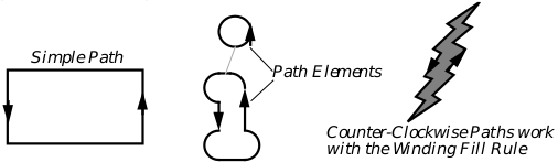
Figure 23-12 Graphics Paths

Paths can be created by taking the intersection or union of two or more paths. In this case, the paths which are combined to make the resulting path are called sub-paths. (See Figure 23-13).

Figure 23-13 Combining Paths

Paths are normally used to describe regions. However, regions are basically bitmaps, whereas paths are described in terms of the standard coordinate space. Thus, while regions don’t scale well at all, it is possible to scale a path perfectly, then use the transformed path to more correctly compute the desired region. If this comparison sounds similar to that between bitmap- and outline- based fonts, it should. The “outline” of an outline-based font character is, in fact, a specialized form of path.

Paths are also used to describe clipping regions. It is possible to combine any path with a window’s clipping region to further restrict the clipping area. Thus it is possible to clip to an ellipse or to a Bézier curve, or even to use text as a clipping region.

Figure 23-14 Geode-Defined Clipping Paths
It is possible to clip using paths incorporating text, splines, and other elements.

When constructing a path, you should keep in mind what it will be used for. If the path is to be filled using the winding rule, it is important that all edges go the correct direction. The winding rule algorithm assumes that the region is described by edges that go around it counterclockwise. Edges going clockwise describe hollows. The odd/even fill rule will work independently of path direction. See section 24.2.11 of chapter 24 for more information about winding rules.

Both the winding and odd/even fill rules demand closed path elements. If any path elements are not filled, the routine will treat them as if they were, connecting the ends of each open path element with a straight line.

It is also possible to alter an existing path by combining it with another. The new path thus formed preserves both paths. If drawn, both paths will appear. If the path is filled or used as a clipping region, the geode can specify how the regions described by the paths should be combined, whether the intersection or union should be taken. Any number of paths can be combined in this manner.

GrBeginPath() signals that the geode is about to start describing a path. All drawing commands directed at the GState will go into constructing the path until GrEndPath() is called. GrBeginPath() is also the routine used to combine a path with an existing path. Calling GrBeginPath() when already constructing a path signals that further graphics commands should describe a new path to be combined with the existing one. The new path can either replace the existing one or combine to find the intersection or the union.

GrCloseSubPath() closes the current path element, adding a straight line segment from the current position to the starting point if necessary.

GrGetPathBounds() returns the bounding coordinates of a rectangle that completely encloses the current path. GrTestPointInPath() tests whether a passed point falls within the current path. GrGetPathPoints() returns all the points along a path in the order visited. GrGetPathRegion() returns the region defined by the path. GrGetPathBoundsDWord() returns the bounds of the path and works in a 32-bit graphics space. If you just want to know whether or not a given path exists, then call GrTestPath(), passing the GetPathType GPT_CURRENT.

GrSetStrokePath() replaces the current path with the one that would result from “stroking” (drawing) the current path with the current line attributes. For example, if the current line style is a dotted line, the result will most likely be a set of many skinny regions. At this time, stroke paths cannot be used for clipping purposes. However, geodes can still draw and fill these paths.

Paths can be drawn or filled using the GrDrawPath() and GrFillPath() commands. For more information about these routines, see section 24.2.11 of chapter 24.

GrGetPath() retrieves the handle of a block containing the path’s data. You may pass this handle to GrSetPath() and thus copy a path to another GState.

23.10 Working With Video Drivers

The main benefit of the device independence is that the geode writer can issue graphics commands without worrying about the device. Working with the video driver is left to the graphics system.

23.10.1 Kernel Routines

GrInvalRect(), GrInvalRectDWord(), GrGrabExclusive(), GrGetExclusive(), GrReleaseExclusive(), GrBitBlt(), GrGetBitmap(), GrGetWinHandle()

Sometimes the geode may want more power over the driver. It can see what device coordinates correspond to a set of standard GEOS coordinates or vice versa.

It is possible to update part of a drawing without exposing the whole window. Calling GrInvalRect() causes a passed rectangular area to be updated; the area outside the rectangle will be unaffected. GrInvalRectDWord() works the same way, but for large coordinate spaces.

Programs can also seize exclusive access to a video driver by calling the GrGrabExclusive() command, which allows only the passed GState to alter what is shown on the screen. This routine is useful for programs such as screen dumps who want to accomplish something concerning the screen without worrying that programs in other threads will change the screen in the meantime. GrReleaseExclusive() ends the exclusive access to the screen so that other GStates can update.

To find out if the video exclusive is presently grabbed, call GrGetExclusive(). This will return the handle of the GState presently in possession of the exclusive, or zero if there is no such GState.

GrBitBlt() is an advanced function used to quickly copy or move data within video memory. Effectively, it can copy or move a rectangular part of the document space to another part of that space-the passed BLTMode will determine whether the area is copied or moved. This might be used in an arcade game or animation program to move simple pictures around the screen very quickly. Pass this function the source and destination rectangles, and whether you are copying or moving the block. After calling GrBitBlt(), the changes have been made to video memory but have not actually been drawn to the screen. Make sure that the affected areas are redrawn by invalidating the appropriate area. If speed is a concern, and if you’re using GrBitBlt() it probably is, you’ll probably want to restrict the clipping area when the drawing is refreshed.

GrGetBitmap() basically returns a dump of an arbitrary display area. It is an advanced function and should be used with some caution. If asked to dump an area from a GState being displayed to screen, GrGetBitmap() won’t check to see if the dumped area is obscured by another window, and so your dump might include a picture of that other window. However, if you’re working with some sort of offscreen bitmap, this function provides a way to look at large portions of it a time. Note that to look at smaller areas, you might prefer to use GrGetPoint(), an optimized, easier to use function to find out the color of a pixel.

At some times, it may prove useful to know what window, if any, is associated with a GState. To find out, call GrGetWinHandle().

23.10.2 Direct Calls to the Driver

Rarely, a geode may wish to make direct calls to the video driver. In most cases, anything your code might want the video driver to do can be handled better by going through the appropriate graphics routine.

23.11 Windowing and Clipping

Windows are the interface between the graphics commands and the GEOS user interface. In this section we will discuss some of the graphical mechanisms associated with windows in GEOS.

23.11.1 Palettes

Each window has a color palette associated with it. For more information about manipulating palettes, see section 24.3.1.3 of chapter 24. The system will use the palette of whatever window is active. As a result, if two windows have different palettes, when one window is active, the other’s colors will be distorted.

23.11.2 Clipping

GrSetClipPath(), GrSetClipRect(), GrGetClipRegion(), GrTestRectInMask(), GrSetWinClipRect(), GrGetMaskBounds(), GrGetMaskBoundsDWord(), GrGetWinBounds(), GrGetWinBoundsDWord()

The graphics system provides some routines which allow geodes to work together with the windowing system to control clipping. A window’s clipping region, you will recall, is that area of the window that must be redrawn. It corresponds to that area of the graphics space which is visible inside the window and not obscured by another window. The area outside the clipping region is supposed to be that area that doesn’t need to be redrawn. Geodes which are certain that part of their graphics space doesn’t need to be (or shouldn’t be) redrawn can restrict their clipping region to exclude this portion.

Restricting the clipping region can lead to quicker redraws, since the graphics system doesn’t have as much to redraw. Arcade games in which most of the action only takes place in one or two areas of the display can restrict their clipping region to speed redraws in the smaller, active areas. Also, the clip region can be used as a sort of stencil (see Figure 23-14).

The clip region is defined by a path which describes the boundaries of the region. A window typically begins with a rectangular clip region. If it is partially obscured by other windows, this rectangle will have “bites” taken out of it. This is done using normal path routines used for combining paths. The clipping path of a newly obscured window is determined by computing its old clipping path with that of the obscuring window.

Since any number of paths may be combined, it is a simple matter for the graphics system to combine a window’s clipping path with a geode’s path chosen to restrict the clipping region. Thus the geode can define its restricted clipping area without knowing anything about the window’s present status.

GrSetClipPath() sets the geode-defined path to use when restricting the window’s clip path. GrSetClipRect() is an optimization of GrSetClipPath() to handle the most common case in which the new path element is a rectangle.

GrGetClipRegion() returns the Region data structure corresponding to the current clip path. GrGetMaskBounds() and GrGetMaskBoundsDWord() return the bounds of the current clipping path.To find out whether there is a clip path at all, just call GrTestPath() and pass GPT_CLIP.

GrTestRectInMask() determines whether a rectangular area lies fully, partially, or not at all within the clipping area. This routine is useful for optimizing redraws.

GrSetWinClipRect() and GrSetWinClipPath() set the clipping path associated with the window; you should never have occasion to use it. GrGetWinBounds() and GrGetWinBoundsDWord() return the bounds of the window clipping path. To find out whether there is a window clipping path at all, call GrTestPath() and pass GPT_WIN_CLIP.

23.11.3 Signalling Updates

GrBeginUpdate(), GrEndUpdate()

The kernel provides two messages by which the geode may signal that it is updating the contents of a window. When updating a region (as when handling a MSG_META_EXPOSED), the geode should call GrBeginUpdate() after creating the GState, and call GrEndUpdate() before destroying the GState.

This causes the system to store the GState for future comparisons during clipping region calculation. If you don’t call these functions, the clipping region is likely to be wrong for this and other updates. Default system MSG_META_EXPOSED handlers call these routines.

Note that you only need call these routines when performing a requested update; if you are drawing to a window without being asked to do so, you need not call these routines.

PCCOM Library <– table of contents –> Drawing Graphics